To use BeamProfiler you must first measure the pdd of the laser
beam you want to analyze, and save it as .csv, .xls, or .xlsx in a known
location. BeamProfiler expects the pdd to comply with the standard
layout to function properly. Below is a description of the standard layout and
an example.
Note
BeamProfiler follows the zero-based indexing.
Header
The header is located in the first row of the pdd file, and it
defines important measurement parameters, which must be present in the
specified locations.
Pixels X:
Number of pixels in the x-axis (R0C5)
Pixels Y:
Number of pixels in the y-axis (R0C8)
Size of windows X:
Measurement window size in the x-axis measured in
millimeter (R0C11)
Size of windows Y:
Measurement window size in the y-axis measured in
millimeter (R0C14)
Null Point:
Value corresponding to the dark-field of the measurement tool
(R0C17)
Body
The body is located from the second row of the pdd file, and it
defines the power density of each individual pixel measured in
ADC/px.
Example
The following table is a truncated pdd that complies with the
standard layout. It has a total of 65,536 pixels (256 pixels in both x-
and y-axis), a measurement window area of approximately 1230 mm2
(35.072 mm in both x- and y-axis), and a null point of 149.063 ADC/px.
If your pdd was measured with the PRIMES LaserDiagnosticsSoftware
v2.98.81, then don’t worry as it already complies with the standard layout.
If your pdd was measured with another software and does not comply with
the standard layout, you have two options:
Modify the pdd so that it matches the standard layout.
Modify the source code so that it reflects your pdd file layout. To access the source code the the Installation section.
Download the example pdd file
lab_beam.xls and save it in a known directory. This pdd
corresponds to a real laser beam used in the laser-assisted bonding process
(LAB). For more information on the LAB process, please refer to the
Theoretical background section. For this example we
will paste the pdd in the
C:\Users\wagnojunior.ab\Desktop\Tutorial\pdd folder.
Important
The auxiliary graphs and the beam analysis report file will be saved in this location.
Start coding
Open your favorite IDE, create a new .py file, and save it in a known
location. For this example we will create a file named example.py and save it in the C:\Users\wagnojunior.ab\Desktop\Tutorial folder. In example.py import BeamProfiler and enter the path to the pdd file and its name as follows:
1importbeamprofiler23# Enter the path to the pdd file and its name4path=r'C:\Users\wagnojunior.ab\Desktop\Tutorial\pdd'5fileName='lab_beam.xls'
We can now move on and set a few user-defined values.
Set the user-defined values
As introduced in the Theoretical background
section, there are three user-defined values that must be set in order to run
BeamProfiler. For this example we will set eta=0.8, epsilon=0.2, and mix=1 in example.py as follows:
7# Set the user-defined values 8eta=0.8 9epsilon=0.210mix=1
With these simple settings we can now leverage the full capabilities of
BeamProfiler.
Run the laser beam characterization
To run the laser beam characterization enter the following lines to example.py and execute the code. The analysis happens when we initialize an instance of type Beam with the function beamprofiler.Beam().
mix (int) – number of normal mixtures used in the normal fit. mix=[1, 2, 3].
Return type:
None.
The variable myBeam is created and all the relevant data related to the beam analysis are saved in it, including the following characterizing
parameters:
ISO parameters:
total power, clip-level power, maximum power density, clip-level
power density, clip-level average power density, clip-level irradiation
area, beam aspect ratio, fractional power, flatness factor, beam
uniformity, plateau uniformity, edge steepness, beam centroid, beam width.
On the next steps we will generate the auxiliary graphs.
Generate the histogram plot
To generate the histogram plot add the following lines to example.py and run the code. The histogram plot is saved when the function beamprofiler.utils.plot.histogram() is called.
histogram plots the histogram of the power density distribution and the
normal mixture fit of the top 40% of the range.
Parameters:
path (std) – path to where the graph will be saved.
fileName (str) – name of the power density distribution file.
beam (Beam) – instance of type Beam.
Other Parameters:
n_bins (int) – number of bins used in the histogram. The default is 256.
zoom (float) – zoom of the inset image. The default is 2.
x1 (float) – lower bound of the inset image on the x-axis. The default is 1600.
x2 (float) – upper bound of the inset image on the y-axis. The default is 2000.
y1 (float) – lower bound of the inset image on the y-axis. The default is 0.
y2 (float) – upper bound of the inset image on the x-axis. The default is 5000.
fmt (str) – image file format.
Return type:
None.
Important
If the kwargs are omitted the histogram is ploted using the default
format. See step 6 for how to customize it
The file lab_beam-histogram.png is created and saved in the
C:\Users\wagnojunior.ab\Desktop\Tutorial\pdd directory. This is a good chance to check if the number of normal mixtures used in the normal fit (variable mix defined in line 10) is appropriate.
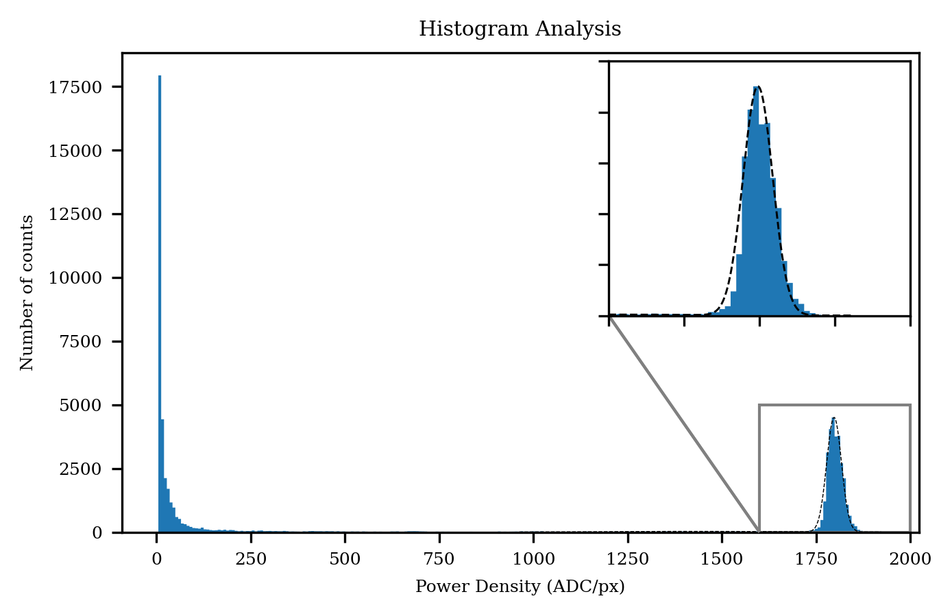
Fig. 6 Default histogram plot for the pdd lab_beam.xls using mix=1
We see that a single Gaussian distribution is not sufficient to fit the data at hand, which results in an unreliable laser beam characterization. Therefore, go back to line 10, change it so that two Gaussian distributions are used instead, and run the code again.
Warning
An ill-fitting normal distribution can negatively affect the soundness of the beam analysis.
15# Generate the histogram plot16kwargs={17'n_bins':512,18'zoom':2.5,19'x1':1600,20'x2':2000,21'y1':0,22'y2':2500,23'fmt':'.png'24}25beamprofiler.utils.plot.histogram(path,fileName,myBeam,**kwargs)
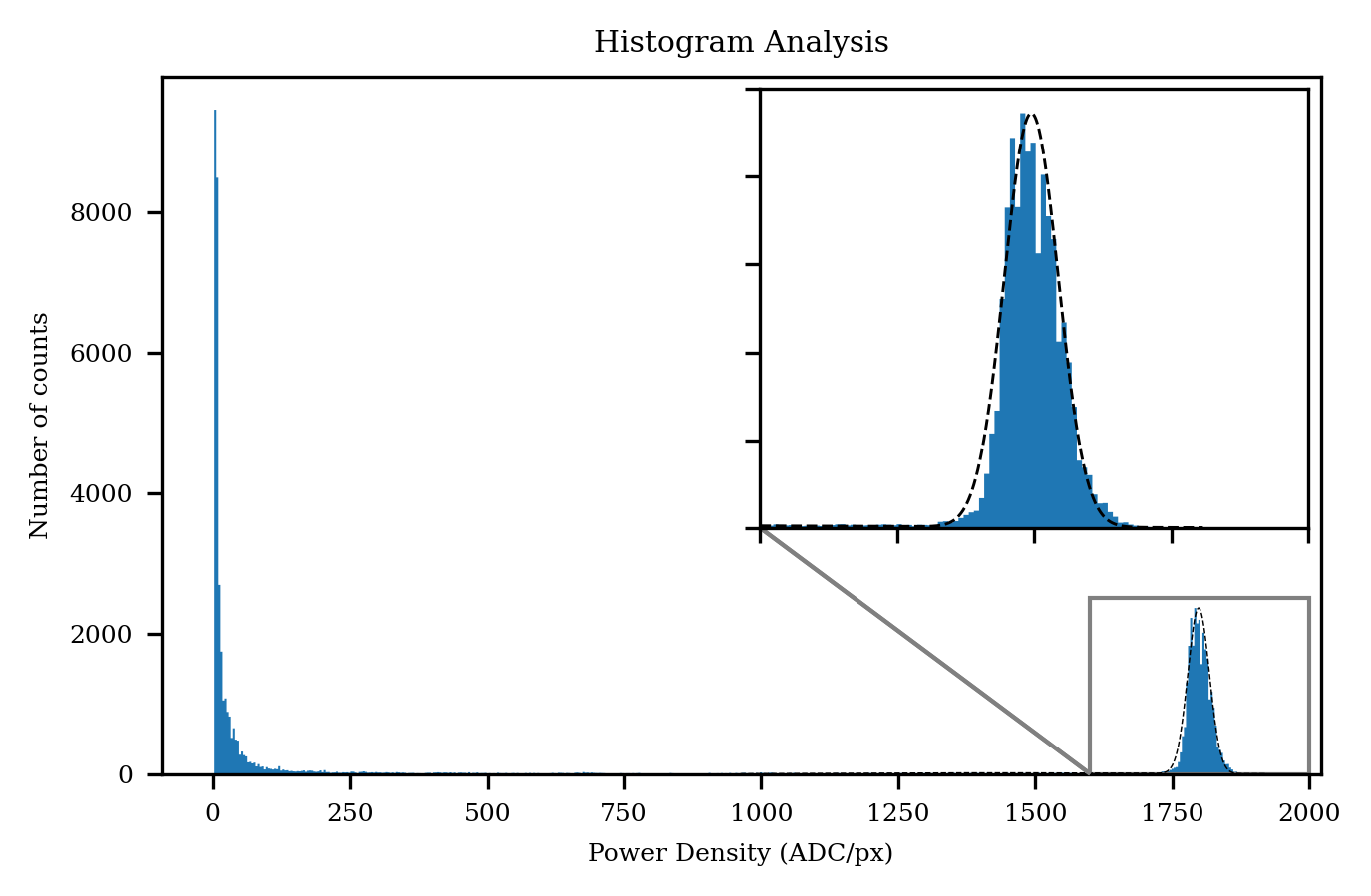
Fig. 8 Customized histogram plot for the pdd lab_beam.xls using mix=2
See the difference? The number of histogram bins n_bins was increased from 256 to 512, the zoom of the inset image was increased from 2 to 2.5, and the top delimiter y2 of the inset image was decreased from 5000 to 2500. The bottom delimiter y1, the left delimiter x1, the right delimiter x2, and the image file format were not changed.
Generate the 2D heat map plot
To generate the 2D heat map plot add the following lines to example.py and run the code. The 2D heat map plot is saved when the function
beamprofiler.utils.plot.heat_map_2d() is called.
27# Generate the 2D heat map plot28beamprofiler.utils.plot.heat_map_2d(path,fileName,myBeam)
heat_map_2d plots the 2D heat map of the power density distribution.
Parameters:
path (str) – path to where the graph will be saved.
fileName (str) – name of the power density distribution file.
beam (Beam) – instance of type Beam.
Other Parameters:
z_lim (float) – upper intensity limit of the cross-section graph of the power density
distribution. The default is -1.
cross_x (float) – x-coordinate of the cross-section graph of the power density
distribution. The default is the calculated beam center about the
x-axis.
cross_y (float) – y-coordinate of the cross-section graph of the power density
distribution. The default is the calculated beam center about the
y-axis.
rect (tuple) – size and position of the reference rectangle. The first two elements of
the tuple define the width and length of the reference rectangle,
repectively. The third and fourth elements of the tuple define the
offset of the reference rectangle relative to the center of the beam.
(width, length, x_offset, y_offset). Default is (0, 0, 0, 0).
fmt (str) – image file format. The default is .png.
Return type:
None.
The file lab_beam-2dheatmap.png is created and saved in the C:\Users\wagnojunior.ab\Desktop\Tutorial\pdd directory. As with the histogram plot, if the kwargs are omitted the 2D heat map is plotted using the default format.
Fig. 9 Default 2D heat map plot for the pdd lab_beam.xls
It is possible to customize the 2D heat map plot by specifying the kwargs values. Go back to line 28, add the following lines, and execute the code.
27# Generate the 2D heat map plot28kwargs={29'z_lim':2500,30'cross_x':20,31'cross_y':20,32'rect':(20,25,0,0),33'fmt':'.png'34}35beamprofiler.utils.plot.heat_map_2d(path,fileName,myBeam,**kwargs)
Fig. 10 Customized 2D heat map plot for the pdd lab_beam.xls
See the difference? The intensity axis was set to 2500, the cross-section point was set to 20mm on both x- and y-axis, and a reference rectangle of size 20×25mm² was added with a zero offset relative to the center of the beam. The image file format was not changed.
Hint
Modify the default kwargs to see the 2D heat map cross-section in a location other than the beam center.
Hint
Modify the default kwargs to add a reference rectangle to the 2D heat map and position it anywhere on the graph.
Attention
rect must be a tuple of size four, otherwise the reference rectangle won’t be ploted.
Generate the 3D heat map plot
To generate the 3D heat map plot add the following lines to example.py and execute the code. The 3D heat map plot is saved when the function beamprofiler.utils.plot.heat_map_3d() is called.
37# Generate the 3D heat map plot38beamprofiler.utils.plot.heat_map_3d(path,fileName,myBeam)
heat_map_3d plots the 3D heat map of the power density distribution.
Parameters:
path (str) – path to where the graph will be saved.
fileName (str) – name of the power density distribution file.
beam (Beam) – instance of type Beam.
Other Parameters:
elev (float) – elevation viewing angle. The default is 50.
azim (float) – azimuthal viewing angle. The default is 315.
dist (float) – distance from the plot. The default is 11.
rect (tuple) – size and position of the reference rectangle. The first two elements of
the tuple define the width and length of the reference rectangle,
repectively. The third and fourth elements of the tuple define the
offset of the reference rectangle relative to the center of the beam.
The fifth element of the tuple defines the offset of the reference
rectangle relative to the z-axis.
(width, length, x_offset, y_offset, z_offset).
Default is (0, 0, 0, 0, 0).
fmt (str) – image file format.
Return type:
None.
The file lab_beam-3dheatmap.png is created and saved in the C:\Users\wagnojunior.ab\Desktop\Tutorial\pdd directory. As with the 2D heat map plot, if the kwargs are omitted the 3D heat map is plotted using the default format.
Fig. 11 Default 3D heat map plot for the pdd lab_beam.xls
It is possible to customize the 2D heat map plot by specifying the kwargs values. Go back to line 38, add the following lines, and execute the code.
37# Generate the 3D heat map plot38kwargs={39'elev':30,40'azim':45,41'dist':15,42'rect':(20,25,0,0,1950),43'fmt':'.png'44}45beamprofiler.utils.plot.heat_map_3d(path,fileName,myBeam,**kwargs)
Fig. 12 Customized 3D heat map plot for the pdd lab_beam.xls
See the difference? The elevation angle was set to 30deg, the azimuthal angle was set to 45deg, the distance was set to 15, and a reference rectangle of size 20×25mm² was added at z=1950 with a zero offset relative to the center of the beam. The image file format was not changed.
Hint
Modify the default kwargs to see the 3D heat map from different angles.
Hint
Modify the default kwargs to add a reference rectangle to the 3D heat map and position it anywhere on the graph.
Attention
rect must be a tuple of size five, otherwise the reference rectangle won’t be ploted.
Generate the normalized energy curve plot
To generate the normalized energy curve plot add the following lines to example.py and execute the code. The normalized energy curve plot is saved when the function beamprofiler.utils.plot.norm_energy_curve() is called.
47# Generate the normalized energy curve plot48beamprofiler.utils.plot.norm_energy_curve(path,fileName,myBeam)
norm_energy_curve plots the normalized energy curve of the power density
distribution.
Parameters:
path (str) – path to where the graph will be saved.
fileName (str) – name of the power density distribution file.
beam (Beam) – instance of type Beam.
Other Parameters:
fmt (str) – image file format.
Return type:
None.
The file lab_beam-energycurve.png is created and saved in the C:\Users\wagnojunior.ab\Desktop\Tutorial\pdd directory.
Fig. 13 Default normalized energy curve plot for the pdd lab_beam.xls
It is possible to customize the normalized energy curve plot by specifying the kwargs values. Go back to line 48, add the following lines, and execute the code.
47# Generate the 3D heat map plot48kwargs={49'fmt':'.svg'50}51beamprofiler.utils.plot.norm_energy_curve(path,fileName,myBeam,**kwargs)
See the difference? The image file format was changed from .pgn to .svg.
Hint
Modify the default kwargs to save the auxiliary graphs in another file format.
Generate the report file
To generate the beam analysis report file add the following lines to example.py and execute the code. The report is saved when the function beamprofiler.utils.report.write()
53# Generate the normalized energy curve plot54beamprofiler.utils.report.write(path,fileName,myBeam)
write writes the beam analysis report in a .xlsx format.
Parameters:
path (str) – directory where the input file is saved.
fileName (str) – name of the input file.
beam (Beam) – object of type Beam.
Return type:
None.
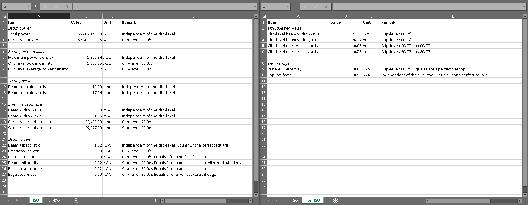
The file BeamAnalysis-lab_beam.xlsx is created and saved in the C:\Users\wagnojunior.ab\Desktop\Tutorial\pdd directory. It includes all the ISO and non-ISO characterizing parameters listed in step 4, and the auxiliary graphs from steps 5–9.
Warning
Only the auxiliary graphs saved in the .png format are included in the report file.
Fig. 14 Beam analysis report for the pdd lab_beam.xls
Review the final code and try it yourself
Most likely the default format of the auxiliary graphs will not be suitable for every pdd, therefore it is important that you are familiar with the customization available in BeamProfiler. Review the final code and try it yourself!
1importbeamprofiler 2 3# Enter the path to the pdd file and its name 4path=r'C:\Users\wagnojunior.ab\Desktop\Tutorial\pdd' 5fileName='lab_beam.xls' 6 7# Set the user-defined values 8eta=0.8 9epsilon=0.210mix=21112# Initialize an instance of type Beam13myBeam=beamprofiler.Beam(path,fileName,eta,epsilon,mix)1415# Generate the histogram plot16kwargs={17'n_bins':512,18'zoom':2.5,19'x1':1600,20'x2':2000,21'y1':0,22'y2':2500,23'fmt':'.png'24}25beamprofiler.utils.plot.histogram(path,fileName,myBeam,**kwargs)2627# Generate the 2D heat map plot28kwargs={29'z_lim':2500,30'cross_x':20,31'cross_y':20,32'rect':(20,25,0,0),33'fmt':'.png'34}35beamprofiler.utils.plot.heat_map_2d(path,fileName,myBeam,**kwargs)3637# Generate the 3D heat map plot38kwargs={39'elev':30,40'azim':45,41'dist':15,42'rect':(20,25,0,0,1950),43'fmt':'.png'44}45beamprofiler.utils.plot.heat_map_3d(path,fileName,myBeam,**kwargs)4647# Generate the normalized energy curve plot48kwargs={49'fmt':'.svg'50}51beamprofiler.utils.plot.norm_energy_curve(path,fileName,myBeam)5253# Generate the report file54beamprofiler.utils.report.write(path,fileName,myBeam)